
Showing posts with label Python. Show all posts

Under the Hood of Apache Airflow: A Guide for Data Engineering

...
engineering information technology
Under the Hood of Apache Airflow: A Guide for Data Engineering

Under the Hood of Apache Airflow: A Guide for Data Engineering

This article provides an in-depth exploration of Data engineering, covering foundational concepts, practical applications, and engineering insights.

Have you ever wondered what actually happens after you write a Python DAG file and save it to your repository? You set a schedule, and like magic, your tasks execute seamlessly every night. However, behind this simple automation lies a powerful, multi-layered architecture that powers modern orchestration.

In the realm of data engineering, Apache Airflow has become the industry standard for managing complex workflows. But to write better pipelines and troubleshoot issues effectively, you need to understand how Airflow works under the hood. Here is a quick breakdown of its core internal components.

1. The DAG Parser: Reading Your Code

When you save a Python file containing a Directed Acyclic Graph (DAG), Airflow doesn't immediately execute your business logic. Instead, the DAG Processor continuously scans your designated DAG folder. It parses the Python script, extracts task dependencies and execution rules, and writes this metadata directly into Airflow’s central metadata database.

2. The Scheduler: The Brain of the Operation

The Airflow Scheduler is the core engine. It constantly monitors the metadata database to check if any tasks are ready to run based on their schedule intervals and upstream dependencies. When a task’s execution time arrives and all prerequisites are satisfied, the Scheduler marks the task as "queued" and hands it off for execution.

3. Executors and Workers: Doing the Heavy Lifting

The Scheduler itself doesn't execute your task code—that responsibility belongs to the Executor and Workers. Depending on your environment (such as Celery or Kubernetes Executors), the Executor determines how task instances are distributed. Worker nodes then pick up the queued tasks, execute the code, and report the final status (success or failure) back to the database.

4. The Webserver: Visualizing the Pipeline

Finally, the Airflow Webserver reads the metadata database to render a clean, interactive user interface. It allows you to inspect DAG structures, monitor real-time execution states, view detailed logs, and trigger manual reruns whenever necessary.

Conclusion

Understanding this continuous cycle—from code parsing to scheduling, execution, and monitoring—is essential for anyone building a career in data engineering. By mastering how these internal components interact, you can design more reliable, scalable, and resilient data pipelines with confidence.

🎬 Related Video Reference

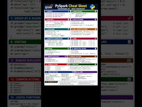
Essential PySpark Commands: The Ultimate Data Engineering Specifications Sheet

...

Building efficient data pipelines requires a solid understanding of PySpark, especially when handling big data workloads. Whether you are transforming massive datasets or building complex ETL workflows, having a structured reference guide ensures your data pipelines run smoothly and adhere to exact technical standards. In big data analytics, treating your code standards and transformations like a detailed engineering specifications sheet can dramatically improve output consistency and speed up development.

Essential PySpark DataFrame Commands for Daily Work

PySpark provides an ideal API for distributed computing, but mastering its vast array of methods can be challenging. To streamline your workflow, every data engineer should maintain a reliable engineering specifications sheet covering fundamental DataFrame operations.

Here are some of the most critical PySpark DataFrame commands you need in your daily toolset:

  • Reading and Writing Data: Master spark.read.format() and df.write.mode() to seamlessly interact with Parquet, CSV, and JSON formats.
  • Data Filtering and Selection: Use select() and filter() (or where()) to isolate key columns and apply conditional logic efficiently.
  • Column Transformations: Employ withColumn() and withColumnRenamed() to modify existing features or create calculated metrics on the fly.
  • Aggregations: Leverage groupBy() alongside built-in SQL functions like count(), sum(), and avg() to extract valuable business insights from raw data.
  • Joining Datasets: Perform high-performance join() operations (inner, left, outer) to merge disparate datasets effectively.

Why Standardizing Your PySpark Operations Matters

By integrating these core PySpark commands into your team's best practices, you eliminate guesswork and optimize query runtime performance. Utilizing this quick-reference guide as your functional engineering specifications sheet for PySpark tasks ensures that your data processing pipelines maintain strict data governance, clean structure, and scalable performance across environments.

Whether you are preparing for a technical data engineering interview or optimizing high-throughput production jobs, keeping these essential PySpark commands top of mind will empower you to write cleaner, faster, and more maintainable Python code.

Technique for Predictive Simulation of Equipment Failures

...

In the era of Industry 4.0, unplanned downtime is the silent killer of productivity. Mastering the Technique for Predictive Simulation of Equipment Failures is no longer a luxury—it is a necessity for competitive manufacturing.

Understanding Predictive Simulation

Predictive simulation combines historical sensor data with machine learning algorithms to forecast when a machine is likely to fail. Unlike traditional preventive maintenance, which follows a rigid schedule, predictive techniques allow for intervention only when necessary, optimizing both cost and uptime.

Key Techniques for Failure Prediction

  • Time-Series Analysis: Using LSTM (Long Short-Term Memory) networks to identify patterns in sensor data over time.
  • Anomaly Detection: Implementing Unsupervised Learning to flag deviations from "normal" operating signatures.
  • Digital Twins: Creating a virtual replica of physical assets to run "what-if" failure scenarios in a risk-free environment.

Implementation Code: Simple Linear Degradation Model

To start with Equipment Failure Simulation, we often look at the Remaining Useful Life (RUL). Below is a conceptual Python snippet using Scikit-Learn to predict failure probability based on operational hours and temperature.


import numpy as np
from sklearn.linear_model import LogisticRegression

# Sample Data: [Operating_Hours, Temperature_Celsius]
X = np.array([[100, 70], [200, 75], [300, 80], [400, 95], [500, 110]])
# Labels: 0 = Healthy, 1 = Risk of Failure
y = np.array([0, 0, 0, 1, 1])

model = LogisticRegression()
model.fit(X, y)

# Predict failure for a machine at 450 hours and 105 degrees
prediction = model.predict_proba([[450, 105]])
print(f"Failure Probability: {prediction[0][1] * 100:.2f}%")

Benefits of Predictive Simulation

By integrating Predictive Simulation into your workflow, you can reduce maintenance costs by up to 30% and eliminate nearly 70% of unexpected breakdowns. The goal is to move from reactive fixing to proactive optimization.

Conclusion

The transition to Predictive Simulation of Equipment Failures requires a robust data pipeline and the right analytical mindset. Start small, monitor your KPIs, and scale your simulation models as your data matures.

Technique for Simulating Machine Degradation Using Sensor Data

...

In the era of Industry 4.0, Predictive Maintenance has become a cornerstone for operational efficiency. However, one of the biggest challenges is the lack of real-world "run-to-failure" data. This is where the Technique for Simulating Machine Degradation Using Sensor Data becomes invaluable for data scientists and engineers.

Why Simulate Machine Degradation?

Simulating degradation allows us to test Remaining Useful Life (RUL) algorithms without waiting months for a machine to actually break. By using mathematical models to generate synthetic sensor readings, we can create diverse failure scenarios and improve model robustness.

The Core Technique: Linear and Exponential Decay

Most industrial assets don't fail instantly. They follow a degradation path. We can simulate this by adding a "health index" that decreases over time, influenced by operational settings and random noise.

import numpy as np
import pandas as pd

def simulate_sensor_degradation(cycles, initial_value, slope, noise_level):
    """
    Simulates a sensor signal with a linear degradation trend.
    """
    time = np.arange(cycles)
    # Linear degradation formula: Value = Initial - (Slope * Time) + Noise
    degradation = initial_value - (slope * time)
    noise = np.random.normal(0, noise_level, cycles)
    
    return degradation + noise

# Example usage: 100 cycles of a temperature sensor
cycles = 100
sensor_data = simulate_sensor_degradation(cycles, initial_value=80, slope=0.15, noise_level=2)
        

Key Components of a Realistic Simulation

  • Baseline Signal: The normal operating range of the sensor (e.g., vibration frequency or temperature).
  • Degradation Trend: Usually modeled using linear, exponential, or Weibull distributions to represent wear and tear.
  • Operational Noise: Random fluctuations (Gaussian noise) that occur in any real-world environment.
  • Anomalous Spikes: Occasional outliers that represent temporary stress on the machine.

Implementing RUL Simulation in Python

To create a dataset for Machine Learning, we often combine multiple simulated sensors. For instance, as a bearing wears down, we might see a simultaneous increase in temperature and vibration levels.

# Generating a sample dataframe for ML training
df = pd.DataFrame({
    'Cycle': np.arange(cycles),
    'Temp_Sensor': simulate_sensor_degradation(cycles, 60, -0.05, 1), # Increasing trend
    'Vibration_Sensor': simulate_sensor_degradation(cycles, 0.5, -0.01, 0.05), # Increasing trend
    'Pressure_Sensor': np.random.normal(100, 2, cycles) # Healthy sensor
})
        

Conclusion

Mastering the Technique for Simulating Machine Degradation is essential for developing reliable Predictive Maintenance systems. By generating high-quality synthetic sensor data, you can bridge the gap between theoretical models and practical industrial applications.

Technique for Regression-Based Remaining Useful Life Prediction

...

In the era of Industry 4.0, predicting when a machine will fail is no longer magic—it's data science. Remaining Useful Life (RUL) prediction is a cornerstone of predictive maintenance, helping industries save millions by preventing unplanned downtime.

What is Regression-Based RUL Prediction?

RUL prediction aims to estimate the time remaining before a component or system fails. Using Regression Analysis, we map historical sensor data (temperature, vibration, pressure) to a continuous time value. Unlike classification, which tells us "if" a machine will fail, regression tells us "when."

Key Techniques in RUL Regression

  • Linear Regression: Best for simple, steady degradation patterns.
  • Random Forest & XGBoost: Excellent for capturing non-linear relationships in complex sensor data.
  • LSTM (Long Short-Term Memory): A deep learning approach that remembers past states, ideal for time-series RUL data.

The Workflow for RUL Modeling

To build an effective regression model for RUL, follow these essential steps:

  1. Data Acquisition: Collect multi-sensor time-series data from healthy to failed states.
  2. Feature Engineering: Calculate rolling means, standard deviations, and trend indicators.
  3. Labeling: Define the target variable (e.g., "Cycles Remaining").
  4. Model Training: Use algorithms like Gradient Boosting to minimize the Root Mean Squared Error (RMSE).

Example: Simple RUL Regression with Python

import pandas as pd
from sklearn.ensemble import RandomForestRegressor

# Load your sensor data
# df = pd.read_csv('sensor_data.csv')

# Feature selection
features = ['sensor_1', 'sensor_2', 'vibration_level']
X = df[features]
y = df['remaining_cycles']

# Initialize and train the model
model = RandomForestRegressor(n_estimators=100)
model.fit(X, y)

print("RUL Prediction Model Trained!")
    

Conclusion

Mastering Regression-Based RUL Prediction allows businesses to move from reactive repairs to proactive optimization. By leveraging machine learning models, engineers can accurately forecast equipment longevity and ensure operational efficiency.

Predictive Maintenance, Regression Analysis, RUL Forecasting, Machine Learning Model, Time-Series Data.

Method for Building Classification Models for Fault Detection

...

In the era of Industry 4.0, Fault Detection has become a cornerstone of operational efficiency. By leveraging machine learning, businesses can predict system failures before they occur. This article outlines a robust method for building classification models for fault detection.

1. Data Acquisition and Preprocessing

The foundation of any classification model is high-quality data. In fault detection, this usually involves sensor readings (temperature, vibration, pressure). Preprocessing steps include:

  • Handling missing values and outliers.
  • Feature Scaling (Standardization or Normalization).
  • Time-series alignment for synchronized sensor data.

2. Feature Engineering

Identifying the right indicators is crucial. Transform raw data into meaningful features using methods like Fast Fourier Transform (FFT) for vibration analysis or statistical features like mean, variance, and kurtosis.

3. Selecting the Classification Algorithm

Choosing the right model depends on the complexity of the fault patterns. Popular choices include:

  • Random Forest: Excellent for handling non-linear data and providing feature importance.
  • Support Vector Machines (SVM): Effective in high-dimensional spaces.
  • Neural Networks (CNN/RNN): Best for complex, sequential sensor data.

4. Implementation Example (Python)

Here is a basic template using Scikit-Learn to build a Random Forest classifier for fault detection:

from sklearn.ensemble import RandomForestClassifier
from sklearn.model_selection import train_test_split
from sklearn.metrics import classification_report

# Load your sensor dataset
# X = features, y = fault_labels
X_train, X_test, y_train, y_test = train_test_split(X, y, test_size=0.2, random_state=42)

# Initialize and train the model
model = RandomForestClassifier(n_estimators=100)
model.fit(X_train, y_train)

# Predictions and Evaluation
predictions = model.predict(X_test)
print(classification_report(y_test, predictions))

5. Evaluation and Deployment

Metrics like Precision, Recall, and F1-Score are vital because fault detection often involves imbalanced datasets (where faults are rarer than normal states). Once validated, the model can be deployed for real-time monitoring via an API or Edge device.

Technique for Detecting Anomalies in Sensor Data Streams

...

In the era of the Industrial Internet of Things (IIoT), the ability to monitor and analyze sensor data streams in real-time is crucial. Identifying irregular patterns—or detecting anomalies—is the key to preventing equipment failure and ensuring operational efficiency.

Understanding Anomaly Detection in Data Streams

Anomaly detection refers to the identification of rare items, events, or observations which raise suspicions by differing significantly from the majority of the data. When dealing with sensor data, we face challenges like high velocity and temporal dependencies.

Top Techniques for Real-Time Detection

  • Statistical Process Control (SPC): Uses mean and standard deviation to identify outliers based on threshold limits.
  • Isolation Forest: An effective unsupervised learning algorithm that isolates anomalies instead of profiling normal points.
  • Long Short-Term Memory (LSTM) Networks: A type of RNN perfect for time-series anomaly detection due to its memory capabilities.

Practical Implementation: Isolation Forest with Python

Below is a simplified conceptual code snippet demonstrating how to implement an anomaly detection model for a continuous stream of sensor readings using the Isolation Forest algorithm.


import numpy as np
from sklearn.ensemble import IsolationForest

# Simulating a stream of sensor data
# Normal data centered around 10, Anomaly at 50
sensor_data = np.array([[10.1], [9.8], [10.5], [50.0], [10.2], [9.9]])

# Initialize the model
# Contamination defines the expected proportion of outliers
model = IsolationForest(contamination=0.1)

# Fit and Predict
model.fit(sensor_data)
predictions = model.predict(sensor_data)

# Result: -1 indicates an anomaly, 1 indicates normal
for i, pred in enumerate(predictions):
    status = "Anomaly" if pred == -1 else "Normal"
    print(f"Reading: {sensor_data[i][0]} -> Status: {status}")

Conclusion

Implementing automated anomaly detection allows businesses to shift from reactive to proactive maintenance. By leveraging machine learning algorithms, you can transform raw sensor streams into actionable insights, ensuring system reliability in any smart environment.

Method for Time-Series Segmentation in Machine Failure Analysis

...

In the era of Industry 4.0, Predictive Maintenance has become a cornerstone of operational efficiency. One of the most critical tasks in this field is Time-Series Segmentation. This process involves partitioning a continuous stream of sensor data into meaningful intervals to identify the precise moment a machine transitions from a normal state to a failure state.

Why Time-Series Segmentation Matters

Machine failure analysis often deals with massive datasets from sensors measuring vibration, temperature, and pressure. Analyzing the entire raw signal is computationally expensive and often noisy. By applying effective segmentation methods, data scientists can:

  • Detect Anomalies faster by focusing on specific change points.
  • Improve the accuracy of Machine Learning models for failure prediction.
  • Extract better features for Root Cause Analysis (RCA).

Key Techniques for Segmentation

There are several algorithmic approaches to segmenting time-series data for failure analysis:

1. Bottom-Up Segmentation

This method starts with the smallest possible segments and merges them based on a cost function until a specific error threshold is reached. It is highly effective for identifying stable operating states.

2. Change Point Detection (CPD)

CPD identifies points in time where the statistical properties of a signal (like mean or variance) change abruptly. This is the "gold standard" for detecting the onset of mechanical wear.

Implementing Segmentation in Python

To perform time-series segmentation, the ruptures library in Python is an excellent tool for offline analysis. Below is a conceptual example of using the Window-based change point detection:


import ruptures as rpt
import numpy as np

# Simulate a machine sensor signal with a change in behavior
signal = np.concatenate([np.random.normal(0, 1, 500), 
                         np.random.normal(5, 2, 500)]) 

# Choose a detection algorithm (Window-based)
algo = rpt.Window(width=40, model="l2").fit(signal)

# Predict the change points (potential failure onset)
result = algo.predict(n_bkps=1)

print(f"Potential Failure Detected at Index: {result[0]}")

Conclusion

Mastering Time-Series Segmentation in Machine Failure Analysis allows engineers to move from reactive repairs to proactive maintenance. By segmenting data effectively, we transform raw sensor noise into actionable insights that save time and reduce costs in industrial environments.

Approach to Handling Missing Sensor Data in Predictive Models

...

In the world of IoT and Industrial 4.0, sensor data is the backbone of predictive maintenance and real-time monitoring. However, "missing data" is an inevitable challenge caused by network instability, battery depletion, or hardware malfunctions. Ignoring these gaps can lead to biased models and inaccurate predictions.

This article explores effective strategies to handle missing sensor data to ensure your predictive models remain robust and reliable.

1. Identifying the Nature of Missingness

Before jumping into solutions, identify why data is missing:

  • MCAR (Missing Completely at Random): No relationship between the missing data and any other values.
  • MAR (Missing at Random): Missingness is related to other observed variables.
  • MNAR (Missing Not at Random): The reason for missingness is related to the missing value itself (e.g., a sensor fails only at high temperatures).

2. Common Imputation Techniques

A. Simple Imputation

For non-critical gaps, filling missing points with the mean, median, or mode of the series is a quick fix. However, this often reduces the variance in your dataset.

B. Time-Series Specific Imputation

Since sensor data is usually sequential, we can use:

  • Forward Fill (Last Observation Carried Forward): Using the last known value to fill the gap.
  • Linear Interpolation: Estimating missing points by drawing a straight line between known values.

C. Advanced Machine Learning Approaches

For complex patterns, use algorithms like K-Nearest Neighbors (KNN) or MICE (Multivariate Imputation by Chained Equations) to predict missing values based on other functioning sensors.

3. Implementation Example (Python)

Here is a quick look at how to handle missing values using the Pandas library:

# Handling missing sensor data in Python
import pandas as pd

# Load your sensor dataset
df = pd.read_csv('sensor_data.csv')

# 1. Linear Interpolation (Best for gradual changes)
df['temperature'] = df['temperature'].interpolate(method='linear')

# 2. Forward Fill (Best for categorical or stable states)
df['status'] = df['status'].ffill()

# 3. Drop rows with too many missing values
df.dropna(thresh=0.8*len(df.columns), inplace=True)
    

Conclusion

Handling missing sensor data is not a one-size-fits-all task. For Predictive Modeling, the goal is to maintain the underlying trend without introducing artificial noise. Start with interpolation, and move to ML-based imputation if the data complexity demands it.

Technique for Feature Scaling and Normalization in Industrial Data

...

Optimizing Machine Learning Models for Industrial Efficiency

In the era of Industry 4.0, Industrial Data comes from various sensors and sources, often with vastly different scales. For instance, temperature might range from 20 to 1000°C, while pressure ranges from 1 to 5 bar. This discrepancy can lead to biased machine learning models. Therefore, mastering Feature Scaling and Normalization is crucial for any data professional.

1. Why Feature Scaling Matters?

Most gradient-based algorithms (like Linear Regression or Neural Networks) and distance-based algorithms (like KNN or SVM) are sensitive to the magnitude of data. Without proper scaling, features with larger values will dominate the learning process, leading to sub-optimal performance.

2. Essential Techniques

Min-Max Normalization

Normalization scales the data into a fixed range, typically 0 to 1. This is particularly useful when you know the distribution of your data does not follow a Gaussian (Normal) distribution.

Formula: $x_{new} = \frac{x - x_{min}}{x_{max} - x_{min}}$

Standardization (Z-score Scaling)

Standardization centers the data around a mean of 0 with a standard deviation of 1. This technique is more robust to outliers, which are common in industrial sensor data.

Formula: $z = \frac{x - \mu}{\sigma}$

3. Python Implementation

Using Scikit-Learn, we can easily apply these techniques to our industrial datasets:


from sklearn.preprocessing import MinMaxScaler, StandardScaler
import pandas as pd

# Sample Industrial Data
data = {'Temperature': [300, 450, 200, 800],
        'Pressure': [1.2, 2.5, 1.1, 4.8]}
df = pd.DataFrame(data)

# Applying Min-Max Scaling
scaler_minmax = MinMaxScaler()
df_normalized = scaler_minmax.fit_transform(df)

# Applying Standardization
scaler_std = StandardScaler()
df_standardized = scaler_std.fit_transform(df)


Conclusion

Choosing between Normalization and Standardization depends on your specific industrial application and the nature of your data. By implementing these Feature Scaling techniques, you ensure that your predictive maintenance and process optimization models are accurate, stable, and reliable.

Technique for Extracting Meaningful Features from Time-Series Sensor Data

...

In the world of IoT and industrial automation, Time-Series Sensor Data is everywhere. However, raw data from sensors like accelerometers or thermometers is often noisy and voluminous. To build effective Machine Learning models, we must transform this raw signal into meaningful features.

Why Feature Extraction Matters?

Raw time-series data is high-dimensional. By extracting features, we reduce dimensionality and highlight the underlying patterns that represent physical phenomena, such as machine vibrations or human movement.

Key Extraction Techniques

  • Time-Domain Features: Statistical measures like Mean, Variance, Kurtosis, and Skewness.
  • Frequency-Domain Features: Using Fast Fourier Transform (FFT) to identify dominant frequencies.
  • Time-Frequency Analysis: Wavelet Transforms for non-stationary signals.

Python Implementation Example

Using pandas and numpy, we can easily extract statistical features from a sensor window.


import numpy as np
import pandas as pd

def extract_features(window):
    """
    Extracts basic statistical features from a time-series window.
    """
    features = {
        'mean': np.mean(window),
        'std_dev': np.std(window),
        'max': np.max(window),
        'min': np.min(window),
        'rms': np.sqrt(np.mean(np.square(window))), # Root Mean Square
        'zero_crossing_rate': ((window[:-1] * window[1:]) < 0).sum()
    }
    return features

# Example: Sensor data from a 100Hz accelerometer
sensor_data = np.random.normal(0, 1, 100)
print(extract_features(sensor_data))

Conclusion

Mastering Feature Extraction is the secret sauce to high-performing predictive maintenance and activity recognition models. By moving from raw data to structured statistical features, you enable your AI to "understand" the physical world more accurately.

Method for Preprocessing Sensor Data for Predictive Maintenance Models

...

In the era of Industry 4.0, Predictive Maintenance (PdM) has become a cornerstone for reducing operational costs. However, the success of any PdM model depends heavily on the quality of input. Raw sensor data is often noisy, inconsistent, and voluminous. This guide explores the essential methods for preprocessing sensor data to build robust predictive models.

Why Preprocessing Matters for Predictive Maintenance

Sensors in industrial machinery often capture data at high frequencies, leading to "dirty data" caused by sensor malfunctions or transmission errors. Without proper cleaning, your Machine Learning model will suffer from the "Garbage In, Garbage Out" syndrome.

Key Steps in Sensor Data Preprocessing

1. Data Cleaning and Handling Missing Values

Sensors may drop signals due to connectivity issues. Common strategies include:

  • Interpolation: Filling gaps based on surrounding data points (Linear or Spline).
  • Mean/Median Imputation: Replacing missing values with statistical averages.

2. Noise Reduction and Smoothing

High-frequency vibrations can create noise. Applying filters helps in extracting the true signal:

  • Moving Average: To smooth out short-term fluctuations.
  • Kalman Filtering: For more complex, dynamic systems.

3. Feature Engineering and Time-Windowing

Predictive maintenance is time-sensitive. Instead of raw data points, we use Time-Windowing to capture trends over time (e.g., the average temperature over the last 24 hours).

Python Implementation Example

Here is a basic snippet using Python and Pandas to preprocess typical sensor data:


import pandas as pd
import numpy as np

# Load sensor dataset
df = pd.read_csv('sensor_data.csv')

# 1. Handling Missing Values using Linear Interpolation
df['temperature'] = df['temperature'].interpolate(method='linear')

# 2. Noise Smoothing using Rolling Mean
df['smooth_vibration'] = df['vibration'].rolling(window=5).mean()

# 3. Feature Engineering: Lag Features
df['prev_pressure'] = df['pressure'].shift(1)

print("Preprocessing Complete!")


Conclusion

Mastering sensor data preprocessing is 80% of the work in Predictive Maintenance. By implementing structured cleaning, filtering, and feature engineering, you ensure that your PdM models are accurate, reliable, and ready for real-world deployment.

Accelerating Innovation: Technique for AI-Assisted Alloy Discovery Using Parallel Computing

...

The quest for new materials—stronger, lighter, and more heat-resistant—is the backbone of modern engineering. Traditionally, alloy discovery took years of trial and error. Today, the integration of Artificial Intelligence (AI) and Parallel Computing is revolutionizing this timeline, allowing researchers to simulate thousands of metal combinations in seconds.

The Challenge of Chemical Complexity

Developing a new alloy involves navigating a massive "compositional space." When you mix five or more elements (High-Entropy Alloys), the possible variations are nearly infinite. This is where AI-assisted alloy discovery becomes essential. Instead of physical testing, we use Machine Learning (ML) models to predict material properties like tensile strength and thermal stability.

Key Concept: By utilizing Parallel Computing, we can distribute these complex ML predictions across multiple GPU/CPU cores, reducing computation time from weeks to hours.

A Modern Workflow for Material Discovery

  1. Data Collection: Gathering historical data from metallurgical databases.
  2. Feature Engineering: Identifying atomic descriptors that influence alloy performance.
  3. Parallel Processing: Using frameworks like MPI or OpenMP to run simulations simultaneously.
  4. AI Optimization: Utilizing Bayesian Optimization to find the "Goldilocks" zone of element ratios.

Why Parallel Computing Matters

In the context of high-performance computing (HPC), parallelization allows the AI to evaluate the energy states of different lattice structures concurrently. If we define the total computational task as $T$, and the number of processors as $P$, the speedup $S$ is ideally represented by:

$$S_p = \frac{T_1}{T_p}$$

This efficiency is what makes real-time material informatics possible, enabling the aerospace and automotive industries to innovate faster than ever before.

Conclusion

The synergy between AI and Parallel Computing is no longer just a luxury—it is a necessity for the next generation of metallurgy. By adopting these AI-assisted techniques, labs can transition from "discovery by chance" to "discovery by design."

Techniques for Integrating Simulation Results into Materials Informatics Platforms

...

In the modern era of R&D, Materials Informatics (MI) has emerged as a cornerstone for accelerating discovery. However, the true power of an MI platform lies in its ability to seamlessly ingest and process simulation results from various computational methods like DFT, Molecular Dynamics, or Phase-field modeling.

Why Integration is the Key to Accelerated Discovery

Integrating computational materials science with data-driven informatics allows researchers to bridge the gap between "virtual experiments" and "big data analytics." By centralizing simulation outputs, teams can apply machine learning (ML) models to predict properties of unseen materials with unprecedented speed.

3 Core Techniques for Seamless Data Integration

1. Standardizing Data Schemas with JSON/XML

One of the primary challenges in materials data management is the variety of output formats. Standardizing these into structured formats like JSON or HDF5 ensures that your materials informatics platform can parse results from different software (e.g., VASP, LAMMPS) without manual intervention.

2. Automated Ingestion via RESTful APIs

To eliminate manual upload errors, use RESTful APIs to automate the flow of data. Once a simulation cluster finishes a job, a script can automatically "push" the results to the MI platform’s database. This ensures real-time data availability for the entire research team.

3. Metadata Enrichment and Provenance Tracking

Raw simulation data is useless without context. Integration techniques must include metadata enrichment—capturing parameters like temperature, pressure, functional used, and software version. This creates a "data lineage" that is essential for reproducible science.

Leveraging Python for Integration

Python remains the gold standard for integrating simulation results. Libraries like Pymatgen or ASE (Atomic Simulation Environment) act as excellent intermediaries to extract data from raw output files and format them for MI databases like MongoDB or PostgreSQL.

Pro Tip: Always implement a validation layer during integration to check for converged vs. non-converged simulation results before they enter your training dataset.

Conclusion

Mastering the integration of simulation results into a Materials Informatics platform is no longer optional—it is a competitive necessity. By focusing on standardization, automation, and rich metadata, organizations can transform fragmented data into a powerful engine for material innovation.

Materials Informatics, Data Integration, Materials Simulation, Python, API, Materials Science, Simulation Techniques, Data Engineering

Method for Automating Metallurgical Simulation Workflows in HTC Environments

...

Optimizing material discovery through high-throughput computing (HTC) and automated digital workflows.

In the modern era of materials science, the demand for rapid metallurgical simulation has grown exponentially. To keep pace with industrial needs, researchers are shifting from manual setups to automated workflows integrated within High-Throughput Computing (HTC) environments.

The Challenges of Manual Simulation

Traditional metallurgical modeling often suffers from human error and low scalability. By implementing an automated metallurgical workflow, labs can process thousands of iterations simultaneously, significantly reducing the time-to-market for new alloys and materials.

Core Methodology for HTC Integration

The transition to an HTC environment requires a robust framework. Here are the essential steps for successful automation:

  • Parameter Space Definition: Identifying key variables in the metallurgical process.
  • Scripting and Orchestration: Using Python or similar languages to manage simulation jobs.
  • Resource Scheduling: Leveraging job schedulers (like Slurm or HTCondor) to distribute tasks across computing nodes.
  • Data Extraction: Automating the post-processing of simulation results for immediate analysis.

Future Outlook

Integrating computational metallurgy with automation is no longer optional. As we move towards Industry 4.0, mastering simulation automation in HTC environments will be the primary driver for innovation in structural and functional materials.

Metallurgy, Automation, Simulation, HTC Computing, Workflow Optimization, Materials Science, Python, Research

Techniques for Automating Electronic Structure Calculations Across Metal Systems

...

Efficiency and precision in computational materials science through automated workflows.

In the rapidly evolving field of computational chemistry, the demand for high-throughput screening of metal systems has never been higher. Understanding the electronic properties of transition metals, alloys, and catalysts requires Electronic Structure Calculations—primarily Density Functional Theory (DFT). However, manual setup and monitoring can be a bottleneck.

Why Automate Metal System Calculations?

Metal systems present unique challenges, such as magnetic configurations and convergence issues. Automating these processes ensures:

  • Consistency: Reducing human error in parameter selection (K-points, pseudopotentials).
  • Scalability: Running hundreds of calculations simultaneously for large-scale material discovery.
  • Data Integrity: Systematic storage of outputs for machine learning integration.

Core Techniques for Automation

1. Workflow Orchestration with AiiDA or Pymatgen

Using Python-based frameworks like AiiDA or Pymatgen allows researchers to build robust pipelines. These tools can automate the generation of input files and handle job submissions to High-Performance Computing (HPC) clusters.

2. Error Handling and Auto-Correction

One of the most powerful techniques is implementing automated error handlers. If a calculation fails to converge due to electronic instability, the script can automatically adjust the smearing parameters or the mixing factor and restart the job.

3. High-Throughput Convergence Testing

Automating the convergence test for plane-wave cutoff energy and K-point grids is essential for ensuring the accuracy of metal system simulations without over-allocating computational resources.

Conclusion

Automating electronic structure calculations is no longer a luxury but a necessity for modern materials science. By leveraging Python libraries and systematic error handling, we can unlock new insights into metal systems with unprecedented speed.

DFT, Electronic Structure, Automation, Metal Systems, Computational Chemistry, Material Science, Python, High-Throughput

Approach to Automated Atomic Configuration Enumeration in Metal Systems

...

In the field of computational materials science, understanding how atoms arrange themselves within a lattice is crucial. Determining the thermodynamic stability and physical properties of alloys requires an automated atomic configuration enumeration. This process involves identifying all possible non-equivalent ways to arrange different types of atoms in a given crystal structure.

Why Automated Enumeration Matters

Manually calculating every possible arrangement in metal systems is nearly impossible due to the combinatorial explosion of configurations. Automated approaches provide:

  • Symmetry Reduction: Using space group symmetry to eliminate redundant configurations.
  • Efficiency: Rapidly generating input for Density Functional Theory (DFT) calculations.
  • Precision: Ensuring no unique configuration is missed in the search space.

The Enumeration Process

The standard approach involves several computational steps. Below is a simplified representation of how an algorithm handles the enumeration of a binary metallic system:

# Conceptual Python Workflow for Atomic Enumeration
import numpy as np
from symmetry_handler import SpaceGroup

def enumerate_configurations(lattice, species):
    # 1. Define the supercell size
    # 2. Apply symmetry operations to find equivalent sites
    # 3. Generate non-equivalent permutations
    # 4. Output the unique atomic coordinates
    pass

# Keywords: Metal Systems, Atomic Lattice, Enumeration Algorithm
    

Key Challenges in Metal Systems

When dealing with complex metal systems, researchers must account for magnetic moments and lattice distortions. The enumeration must be robust enough to handle high-entropy alloys (HEAs) where the number of chemical species exceeds four or five, significantly increasing the complexity of the atomic configuration search.

Conclusion

Automating the enumeration of atomic configurations is a cornerstone of modern high-throughput materials discovery. By leveraging symmetry and efficient algorithms, we can explore the vast chemical space of metals with unprecedented speed and accuracy.


Materials Science, Computational Chemistry, Atomistic Simulation, Metal Systems, Python, Atomic Configuration, Automation, Enumeration

Method for High-Throughput Atomic Structure Generation in Metallurgical Research

...

Exploring the frontier of computational materials science through automated structural modeling.

In the modern era of metallurgical research, the ability to rapidly design and test new alloys is crucial. Traditional trial-and-error methods are being replaced by High-Throughput (HT) computational techniques. This article discusses the methodology for generating thousands of atomic structures efficiently, a key step in accelerating material discovery.

The Importance of High-Throughput Atomic Modeling

The core of computational metallurgy lies in understanding the arrangement of atoms. High-throughput atomic structure generation allows researchers to:

  • Scan vast chemical spaces for stable alloy phases.
  • Provide massive datasets for Machine Learning (ML) training in materials science.
  • Simulate thermodynamic properties of complex metallic systems.

Key Methodology: From Algorithms to Atoms

Generating structures at scale requires a robust workflow. Typically, this involves using Python-based libraries such as ASE (Atomic Simulation Environment) or Pymatgen. The process follows these critical steps:

  1. Symmetry Definition: Selecting Space Groups and Lattice Parameters.
  2. Elemental Substitution: Systematically replacing atoms to create different chemical compositions.
  3. Geometry Optimization: Using Density Functional Theory (DFT) or Interatomic Potentials to relax the generated structures.

The Role of Automation in Metallurgy

By automating atomic structure generation, we minimize human error and significantly reduce the time required to identify high-performance materials. Whether it's for high-entropy alloys or next-generation superconductors, high-throughput methods are the engine of modern innovation.

Conclusion

Adopting high-throughput methods in metallurgical research is no longer optional—it is a necessity. As computational power increases, our ability to predict and engineer the atomic world will lead to a new age of material efficiency.

Metallurgy, Atomic Structure, High-Throughput, Computational Materials Science, Python, Research Methodology, Crystal Structure

Technique for Automating Large-Scale Atomic Structure Screening in Metallurgy

...

In the rapidly evolving field of computational metallurgy, the ability to rapidly identify promising materials is a game-changer. Manual analysis of atomic arrangements is no longer feasible when dealing with thousands of potential alloys. Today, we explore the essential techniques for automating large-scale atomic structure screening to accelerate material discovery.

1. High-Throughput Screening (HTS) Frameworks

The foundation of automation lies in High-Throughput Screening. By utilizing Python-based libraries such as ASE (Atomic Simulation Environment) and Pymatgen, researchers can programmatically generate and manipulate atomic structures. This allows for the systematic variation of lattice parameters and dopant concentrations without manual intervention.

2. Integrating Density Functional Theory (DFT) Workflows

To predict the stability of a metallic structure, integrating Density Functional Theory (DFT) calculations into your automation pipeline is crucial. Using workflow managers like AiiDA or Fireworks, you can automate the submission of thousands of jobs to high-performance computing (HPC) clusters, ensuring that atomic structure screening is both continuous and error-free.

3. Machine Learning and Pattern Recognition

Once the raw data is generated, the next step in metallurgy automation is filtering the results. Modern techniques involve training Machine Learning (ML) models to recognize stable patterns in atomic descriptors. This significantly reduces the computational cost by bypassing expensive simulations for structures that the model predicts to be unstable.

"Automation in metallurgy isn't just about speed; it's about exploring the vast chemical space that was previously unreachable."

Key Benefits of Automated Screening:

  • Scalability: Analyze millions of atomic configurations simultaneously.
  • Consistency: Eliminate human error in data entry and structural setup.
  • Data-Driven Discovery: Leverage big data to find unconventional metallic properties.

Conclusion

Adopting an automated atomic structure screening technique is essential for any modern metallurgical laboratory. By combining Python scripting, HPC-based DFT workflows, and Machine Learning, we can transform how we design the next generation of high-performance alloys.

Metallurgy, Atomic Structure, Automation, Python, Materials Science, Machine Learning, High-Throughput Screening, DFT

Leveraging IT Engineering for Real-Time Data Optimization

...


Harnessing IT Engineering for High-Efficiency Real-Time Data Optimization

In the modern digital landscape, real-time data optimization has transitioned from a luxury to a technical necessity. By leveraging advanced IT engineering principles, organizations can transform raw data streams into actionable insights instantly.

The Role of Stream Processing

To achieve optimal performance, engineers must implement robust pipelines. Below is a practical example using Python and Kafka. This snippet demonstrates how to ingest and process data packets in real-time, ensuring minimal latency.

Python
import json
from kafka import KafkaConsumer, KafkaProducer

# IT Engineering: Initializing Real-Time Data Pipeline
def optimize_data_stream():
    # Define consumer for incoming raw data
    consumer = KafkaConsumer(
        'raw-data-topic',
        bootstrap_servers=['localhost:9092'],
        value_deserializer=lambda m: json.loads(m.decode('utf-8'))
    )

    # Define producer for optimized output
    producer = KafkaProducer(
        bootstrap_servers=['localhost:9092'],
        value_serializer=lambda v: json.dumps(v).encode('utf-8')
    )

    print("Status: System Online. Monitoring real-time streams...")

    for message in consumer:
        raw_payload = message.value
        
        # Optimization Logic: Filtering and Data Transformation
        if raw_payload.get('status') == 'active':
            optimized_data = {
                'id': raw_payload['id'],
                'timestamp': raw_payload['ts'],
                'value': round(raw_payload['val'], 2), # Data Optimization step
                'processed': True
            }
            
            # Pushing to optimized stream
            producer.send('optimized-data-topic', optimized_data)
            print(f"Optimization Complete: {optimized_data['id']}")

if __name__ == "__main__":
    optimize_data_stream()

Why This Matters

Effective data optimization reduces server overhead and improves the speed of decision-making. By refining data at the ingestion point, IT engineers ensure that downstream applications receive only the most relevant, high-quality information.

IT Engineering, Real-Time Data, Data Optimization, Python, Kafka, Stream Processing, Tech Tutorial